Teaching
Urban Analytics (ITAO 40570 / MSBR 70580)
ML in Urban Analysis
Spring 2023, 2024 (Elective for Real Estate Minor)
1. Data Preparation and Exploratory Data Analysis (EDA)
Citi Bike
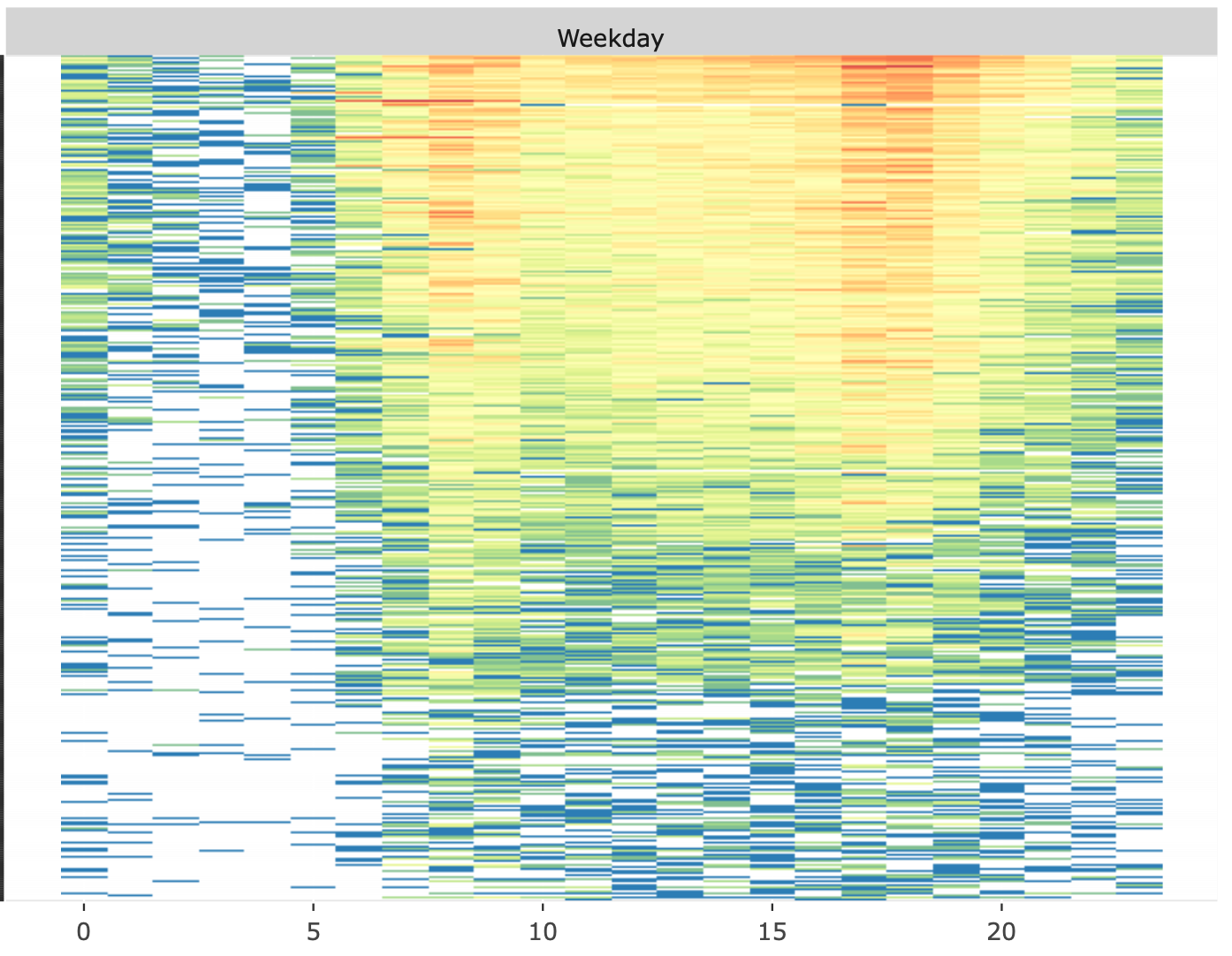
Data Science is a field of science connecting statistics, computer science, and domain knowledge. We would like to discover the pattern of differences and changes, as well as the reasons behind the scene. For any well-designed study, we need to first layout the goal of the study. Using domain knowledge we may list possible factors related to the study, i.e., we need to first design what information may help us to achieve the goal. Taking feasibility and cost into account, we will come up with a list of variables and then gather data (from experiments, surveys, or other studies). On the other hand we may want to learn important insights from existing data. Both the quantity and quality of data determine the success of the study. Once we have the data, we proceed to extract useful information. To use the data correctly and efficiently we must understand the data first. In this lecture, we go through some basic data acquisition/preparation and exploratory data analysis to understand the nature of the data, and to explore plausible relationships among the variables.
Data Science is a field of science connecting statistics, computer science, and domain knowledge. We would like to discover the pattern of differences and changes, as well as the reasons behind the scene. For any well-designed study, we need to first layout the goal of the study. Using domain knowledge we may list possible factors related to the study, i.e., we need to first design what information may help us to achieve the goal. Taking feasibility and cost into account, we will come up with a list of variables and then gather data (from experiments, surveys, or other studies). On the other hand we may want to learn important insights from existing data. Both the quantity and quality of data determine the success of the study. Once we have the data, we proceed to extract useful information. To use the data correctly and efficiently we must understand the data first. In this lecture, we go through some basic data acquisition/preparation and exploratory data analysis to understand the nature of the data, and to explore plausible relationships among the variables.
2. Spatial Data
Citi Bike
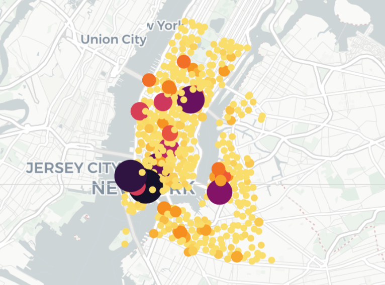
One of the fundamental challenges in the urban analysis is the spatial relationships among the observations. The first step to understanding the spatial relationship is to understand how to operate spatial data and visualize the spatial structure. It is also imperative to associate the data of interest with their location. As pervasive geographic data are becoming available in cities around the world, we need to equip ourselves with proper toolkits.
In this lecture, we will continue with the Citi bike case study from the last lecture. We will study how to visualize the bike stations and the trips. Then we will introduce the common data structure for spatial data – simple feature access, a standard that is used in many geographical information systems (GIS), and the sf package.

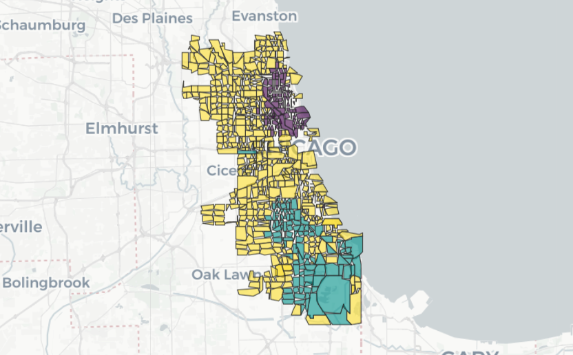
3. Spatial Networks: Network, Centrality, Clustering
Citi Bike, NYC Bike Network
Networks are ubiquitous in our daily life and play a crucial role in our lives – social networks, social media, economic networks, transportation networks, you name it. Networks, to be specific, are used to represent the relationships between the objects of interest. The study of networks dates back to the 18th by Euler and the United States National Research Council defines network science as “the study of network representations of physical, biological, and social phenomena leading to predictive models of these phenomena.” The research on network is still very active today.
As we have seen in previous lectures, urban phenomena can be also represented using networks, such as bike trips and bike routes. There is also a surge in the application of network analysis methods in urban and regional studies in the past decade. Research has shown that network analysis measures can be useful predictors for a number of interesting urban phenomena and can provide insights into wider sociological, economical and geographic factors in certain areas. For our Citibike case study, our goal of this lecture is to study:
1. Where are the centers of the bike network?
2. What are the clusters?
The methods we introduce in this lecture is general and can be applied to other type of networks as well.
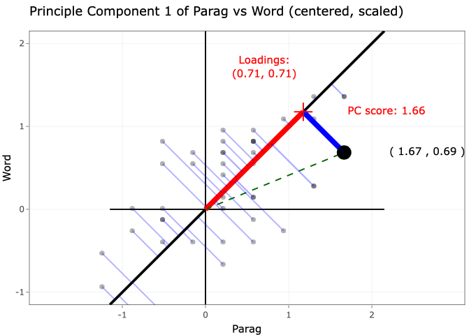
4. Principal Component Analysis
AirBnB
Massive data is easily available to us. How can we efficiently extract important information from a large number of features or variables which will possess the following nice properties:
1. Dimension reduction/noise reduction: They are “closed” to the original variables but only with a few newly formed variables.
2. Grouping variables/subjects efficiently: They will reveal insightful grouping structures.
3. Visualization: we can display high dimensional data.
Principle Component Analysis is a powerful method to extract low dimension variables. One may search among all linear combinations of the original variables and find a few of them to achieve the three goals above. Each newly formed variable is called a Principle Component. PCA is closely related to Singular Value Decomposition (SVD). Both PCA and Singular Value Decomposition are successfully applied in many fields such as face recognition, recommendation system, text mining, Gene array analyses among others. PCA is unsupervised learning. There will be no responses. It works well in clustering analyses. In addition, PCs can be used as input in supervised learning as well.

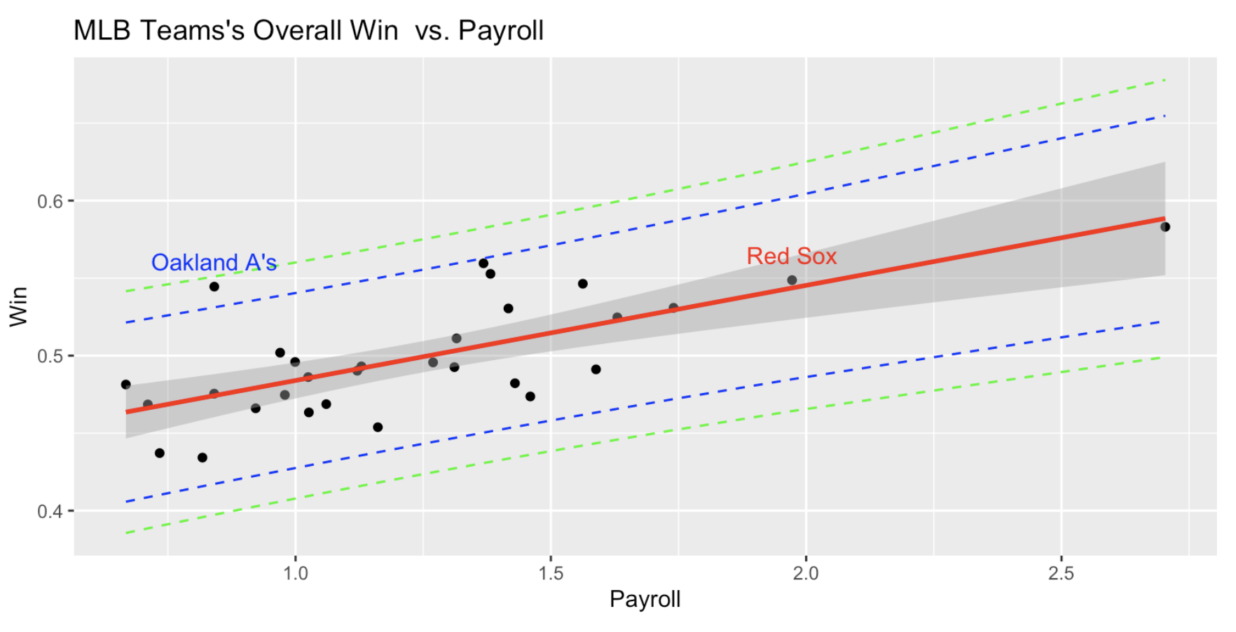
5. Regression
Chicago House Price
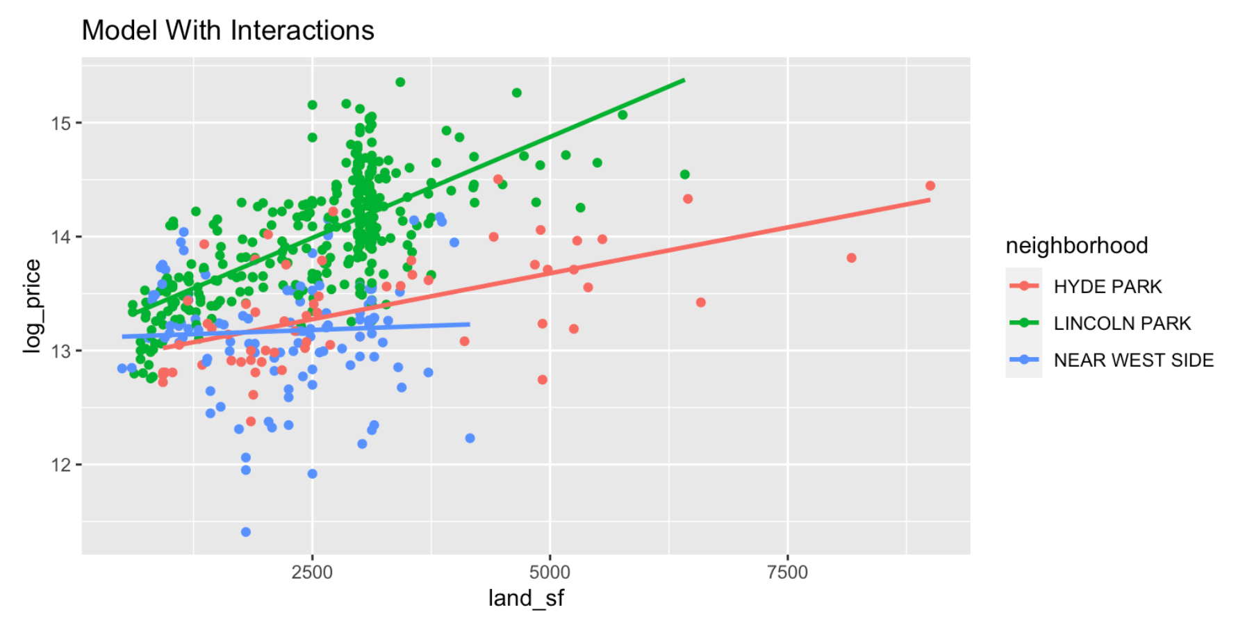
Data Science is a field of science. We try to extract useful information from data. In order to use the data efficiently and correctly we must understand the data first. According to the goal of the study, combining the domain knowledge, we then design the study. In this lecture we first go through some basic explore data analysis to understand the nature of the data, some plausible relationship among the variables.
Data mining tools have been expanded dramatically in the past 20 years. Linear model as a building block for data science is simple and powerful. We introduce/review linear models. The focus is to understand what is it we are modeling; how to apply the data to get the information; to understand the intrinsic variability that statistics have.
6. Large Data, Sparsity and LASSO
Crime Rate, COVID-19
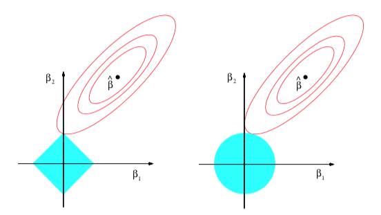
Linear model with least squared estimates are simple, easy produce and easy interpret. It often works well for the purpose of prediction. However when there are many predictors it is hard to find a set of "important predictors". In addition, when the number of predictors p is larger than the number of the observations n we can not estate all the coefficients. In this lecture we introduce LASSO (Least Absolute Shrinkage and Selection Operator) to produce a sparse model. One may view LASSO as a model selection scheme. K-Fold Cross Validation Errors will be introduced and used. [Figure source Hastie et al. (2009)]
Linear model with least squared estimates are simple, easy produce and easy interpret. It often works well for the purpose of prediction. However when there are many predictors it is hard to find a set of "important predictors". In addition, when the number of predictors p is larger than the number of the observations n we can not estate all the coefficients. In this lecture we introduce LASSO (Least Absolute Shrinkage and Selection Operator) to produce a sparse model. One may view LASSO as a model selection scheme. K-Fold Cross Validation Errors will be introduced and used. [Figure source Hastie et al. (2009)]
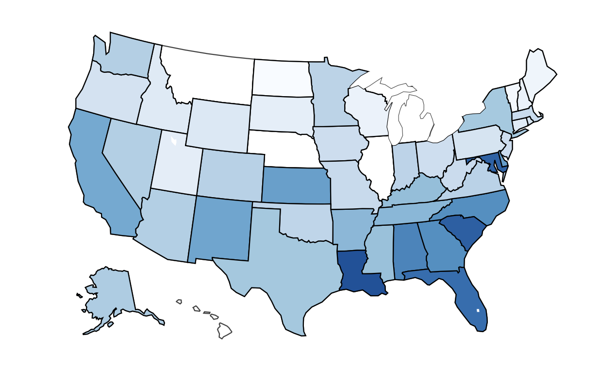
7. Spatial Regression
Chicago House Price
Classical regression assumes the data is independent, while we have seen in spatial data and spatial network lectures, observations are often related with each other. In particular, “everything is related to everything else, but near things are more related than distant things.” – the first law of geography by Waldo Tobler. It is, therefore, important to account for the correlation between near things.
To quantify the relationships between things/observations, we use the concept of spatial autocorrelation. Spatial regression, on the other hand, is a method that takes spatial autocorrelation into account when modeling the relationship between variables.
8. Classification
Fannie May
What are the important risk factors of default for mortgage lenders to decide whether they should approve the loan? What determines an employee being a desirable one for the firm? What are possible risk factors related to heart diseases? How to model a categorical variable conveniently and efficiently? Logistic regression model are the most commonly used methods to model the probability of an event. We then automatically get a linear classification rules. Various criteria are introduced. Analogous to least squared solutions for the usual regression models, we use maximum likelihood estimations.
What are the important risk factors of default for mortgage lenders to decide whether they should approve the loan? What determines an employee being a desirable one for the firm? What are possible risk factors related to heart diseases? How to model a categorical variable conveniently and efficiently? Logistic regression model are the most commonly used methods to model the probability of an event. We then automatically get a linear classification rules. Various criteria are introduced. Analogous to least squared solutions for the usual regression models, we use maximum likelihood estimations.
9. Text Mining
Yelp Review
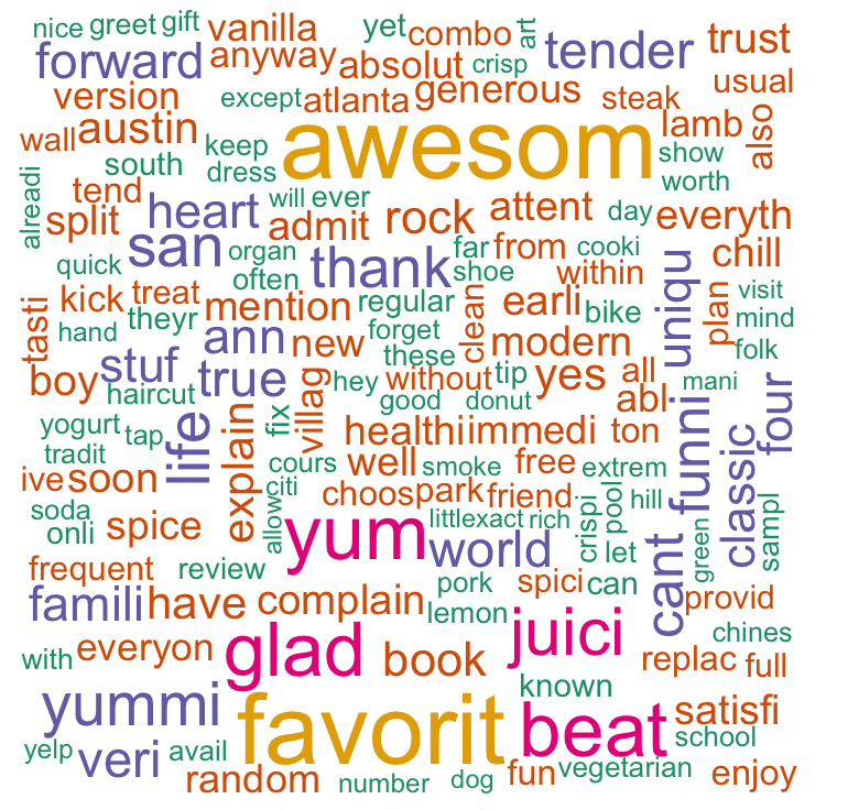
In modern data mining, we often encounter the situation where a text may contain important, useful information about response of interest. Can we predict how much one likes a movie, a restaurant or a product based on his/her reviews? One simple but effective way of learning from a text is through bag of words to convert raw text data into a numeric matrix. We first turn each text into a vector of frequency of words. The bag of words approach can be extended using the n-gram or k-skip-n-gram techniques to account for the semantics of word ordering. Then we apply existing methods that use numerical matrices to either extract useful information or carry out predictions. We will extend the regularization technique (LASSO) to classification problems.
In this lecture through the Yelp case study, we will use the tm package to transform text into a word frequency matrix. We will build a classifier and conduct sentiment analysis. Finally we build a word cloud to exhibit words for good reviews and bad reviews respectively.

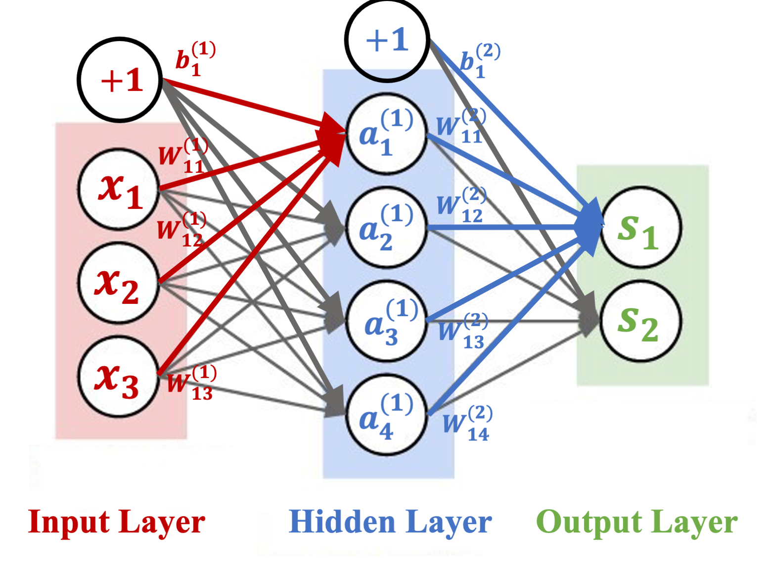
10. Neural Network / Deep Learning
Yelp Review / MNIST CIFAR10
This lecture provides an introduction to Neural Network and Convolutional Neural Network. We will see how neural network borrows the idea of cognitive science and models the behavior of neurons so as to mimic the perception process of human being. On high level, Neural Network is a “parametric” model with huge number of unknown parameters. It is easy to understand the entire set up with knowledge of regressions. Thank to the CS people who has been developing efficient, fast computation algorithm we are able to estimate millions unknown parameters within no time.
Though the neural network model is easy for us to understand but there are a set of new terminologies introduced. Based on the neural network model, we will set up the architecture (model specification) with input layer, hidden layers and output layer and apply the package to several case studies. A well known case study MNIST will be carried out here through the basic NN.
11. Large Language Model (LLM)
Yelp Review
In modern data mining, we often encounter the situation where a text may contain important, useful information about response of interest. In this module, we will cover how to use LLMs and Transformers to analyze text data. Specifically, we will use the HuggingFace transformer pipeline in order to perform sentiment analysis on a given text. We will also use the Transformer models to answer questions based on the text data. Finally, we will use the pipelines in order to summarize the text.
Google Drive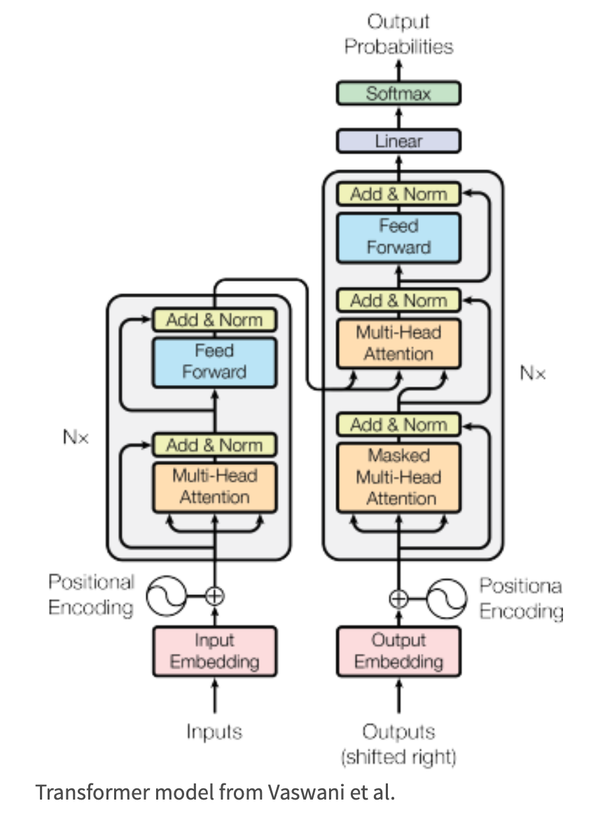
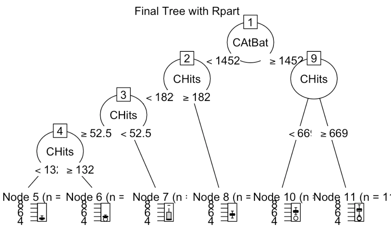
12. Decision Trees and Random Forest
Chicago House Price
Regression combining with regularization works for many studies, especially in the case where we try to identify important attributes. Its simple interpretation and well established theory makes the method classical and useful. On the other hand the strong model assumptions may not be met.
For the purpose of prediction, a model free approach may gain more in accuracy. We start with decision trees. The predictors will be partitioned into boxes. Sample mean in each box is the predicted value for all the subjects in the box. While wild search of optimal boxes is impossible, we use binary, top-down, greedy, recursive algorithm to build a tree. It enjoys the simplicity, easy to interpret. Interactions can be detected through the tree. On the other hand the greedy search is unnecessarily providing the global optimal solution. Also a tree can easily overfit. While the training error is small, the variance is also big. As a result the testing error may suffer.
To reduce the prediction error from a single equation, one idea is to take the average of many very different perdition equations. Bagging and Random Forest are proposed to aggregate many Bootstrap trees. To make trees uncorrelated, a single random tree is built by randomly take m many variables to be split at each node.
In general, we want to bag MANY different equations. They can be completely different methods, such as linear model, lasso equations with different lambda, random forests with different mtry, split predictors.
Decision trees, bagging and random forests are all readily/easily extended to classification problems. To build a tree we use sample proportions to estimate the probability of the outcome, instead of sample means. The criteria choosing the best split can be entropy, gini index and misclassification errors.
Modern Data Mining
This is a cross-listed course with a student body mixed with advanced undergraduates, masters, MBAs, and Ph.D.s. The course covers data science essentials -- a wide selection of supervised and unsupervised learning methods and keeps pace with state-of-the-art methods. It focuses on the statistical ideas and machine learning methodologies that will equip students to analyze modern complex and large-scale data.
This is a cross-listed course with a student body mixed with advanced undergraduates, masters, MBAs, and Ph.D.s. The course covers data science essentials -- a wide selection of supervised and unsupervised learning methods and keeps pace with state-of-the-art methods. It focuses on the statistical ideas and machine learning methodologies that will equip students to analyze modern complex and large-scale data.
1. Data Preparation and Exploratory Data Analysis (EDA)
Data Science is a field of science connecting statistics, computer science, and domain knowledge. We would like to discover the pattern of differences and changes, as well as the reasons behind the scene. For any well-designed study, we need to first layout the goal of the study. Using domain knowledge we may list possible factors related to the study, i.e., we need to first design what information may help us to achieve the goal. Taking feasibility and cost into account, we will come up with a list of variables and then gather data (from experiments, surveys, or other studies). On the other hand we may want to learn important insights from existing data. Both the quantity and quality of data determine the success of the study. Once we have the data, we proceed to extract useful information. To use the data correctly and efficiently we must understand the data first. In this lecture, we go through some basic data acquisition/preparation and exploratory data analysis to understand the nature of the data, and to explore plausible relationships among the variables.
Data Science is a field of science connecting statistics, computer science, and domain knowledge. We would like to discover the pattern of differences and changes, as well as the reasons behind the scene. For any well-designed study, we need to first layout the goal of the study. Using domain knowledge we may list possible factors related to the study, i.e., we need to first design what information may help us to achieve the goal. Taking feasibility and cost into account, we will come up with a list of variables and then gather data (from experiments, surveys, or other studies). On the other hand we may want to learn important insights from existing data. Both the quantity and quality of data determine the success of the study. Once we have the data, we proceed to extract useful information. To use the data correctly and efficiently we must understand the data first. In this lecture, we go through some basic data acquisition/preparation and exploratory data analysis to understand the nature of the data, and to explore plausible relationships among the variables.
2. Principal Component Analysis
Massive data is easily available to us. How can we efficiently extract important information from a large number of features or variables which will possess the following nice properties:
1. Dimension reduction/noise reduction: They are “closed” to the original variables but only with a few newly formed variables.
2. Grouping variables/subjects efficiently: They will reveal insightful grouping structures.
3. Visualization: we can display high dimensional data.
Principle Component Analysis is a powerful method to extract low dimension variables. One may search among all linear combinations of the original variables and find a few of them to achieve the three goals above. Each newly formed variable is called a Principle Component. PCA is closely related to Singular Value Decomposition (SVD). Both PCA and Singular Value Decomposition are successfully applied in many fields such as face recognition, recommendation system, text mining, Gene array analyses among others. PCA is unsupervised learning. There will be no responses. It works well in clustering analyses. In addition, PCs can be used as input in supervised learning as well.
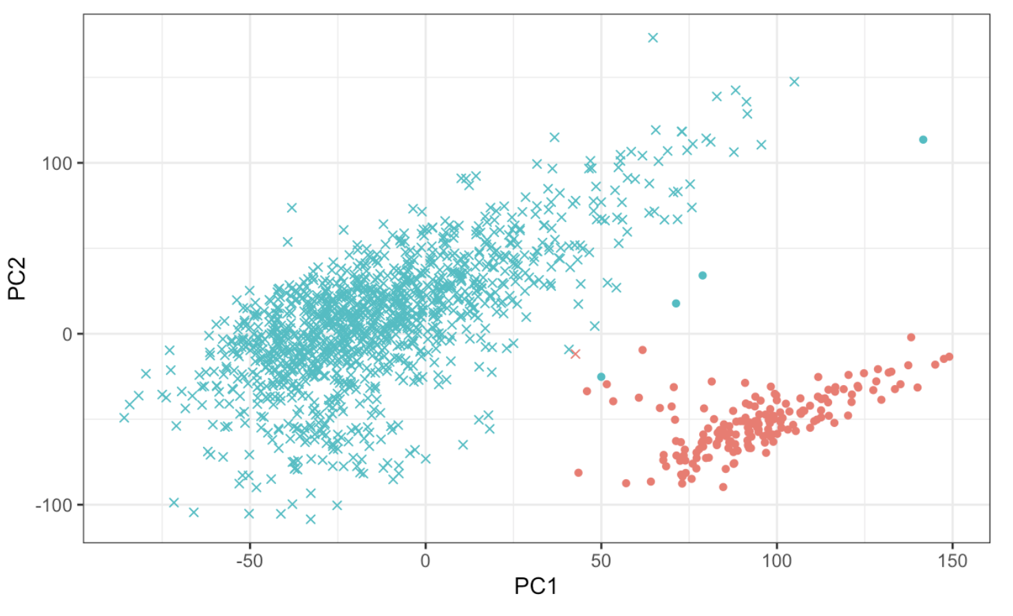
3. Clustering Analysis
Clustering is the task of grouping together a set of objects in a way that objects in the same cluster are more similar to each other than to objects in other clusters. Similarity is an amount that reflects the strength of relationship between two data objects. Clustering is mainly used for exploratory data mining. It is used in many fields such as machine learning, pattern recognition, image analysis, information retrieval, bioinformatics, data compression, and computer graphics.
Given a set of features X1,X2,...,Xp measured on n observations, the goal is to discover interesting things about the measurements on X1,X2,...,Xp. Is there an informative way to visualize the data? Can we discover subgroups among the variables or among the observations?
Among many methods, k-means and Hierarchical clustering are most commonly used. We will go in depth with k-means and leave Hierarchical clustering method for students to study. We will demonstrate the power of using PCA to lower dimension for clustering via an mRNA sequencing case study.
4. Regression
Data Science is a field of science. We try to extract useful information from data. In order to use the data efficiently and correctly we must understand the data first. According to the goal of the study, combining the domain knowledge, we then design the study. In this lecture we first go through some basic explore data analysis to understand the nature of the data, some plausible relationship among the variables.
Data mining tools have been expanded dramatically in the past 20 years. Linear model as a building block for data science is simple and powerful. We introduce/review linear models. The focus is to understand what is it we are modeling; how to apply the data to get the information; to understand the intrinsic variability that statistics have.
5. Model Selection
Multiple regression is a simple yet powerful tool in statistics and machine learning. When we have a number of predictors available, searching for a model that is parsimonious yet good becomes necessary. Sometimes we even have the situation that number of predictors are larger than the sample size. In such cases we can not find unique least squared estimators in a linear model. In this lecture we introduce a model selection treatment by first defining model accuracy such as Prediction Errors. We then propose the commonly used statistics Cp, BIC and AIC and Testing Errors to help choose a good model. A function Regsubsets by leaps are used to do model selection. A complete case study to predict baseball players will be done.
Multiple regression is a simple yet powerful tool in statistics and machine learning. When we have a number of predictors available, searching for a model that is parsimonious yet good becomes necessary. Sometimes we even have the situation that number of predictors are larger than the sample size. In such cases we can not find unique least squared estimators in a linear model. In this lecture we introduce a model selection treatment by first defining model accuracy such as Prediction Errors. We then propose the commonly used statistics Cp, BIC and AIC and Testing Errors to help choose a good model. A function Regsubsets by leaps are used to do model selection. A complete case study to predict baseball players will be done.
6. Large Data, Sparsity and LASSO
Linear model with least squared estimates are simple, easy produce and easy interpret. It often works well for the purpose of prediction. However when there are many predictors it is hard to find a set of "important predictors". In addition, when the number of predictors p is larger than the number of the observations n we can not estate all the coefficients. In this lecture we introduce LASSO (Least Absolute Shrinkage and Selection Operator) to produce a sparse model. One may view LASSO as a model selection scheme. K-Fold Cross Validation Errors will be introduced and used. [Figure source Hastie et al. (2009)]
Linear model with least squared estimates are simple, easy produce and easy interpret. It often works well for the purpose of prediction. However when there are many predictors it is hard to find a set of "important predictors". In addition, when the number of predictors p is larger than the number of the observations n we can not estate all the coefficients. In this lecture we introduce LASSO (Least Absolute Shrinkage and Selection Operator) to produce a sparse model. One may view LASSO as a model selection scheme. K-Fold Cross Validation Errors will be introduced and used. [Figure source Hastie et al. (2009)]

7. Classification
What are possible risk factors related to heart diseases? What determines an employee being a desirable one for the firm? How to tell wehther a review in Amazon is real or not? How to model a categorical variable conveniently and efficiently? Logistic regression model are the most commonly used methods to model the probability of an event. We then automatically get a linear classification rules. Various criteria are introduced. Analogous to least squared solutions for the usual regression models, we use maximum likelihood estimations.
What are possible risk factors related to heart diseases? What determines an employee being a desirable one for the firm? How to tell wehther a review in Amazon is real or not? How to model a categorical variable conveniently and efficiently? Logistic regression model are the most commonly used methods to model the probability of an event. We then automatically get a linear classification rules. Various criteria are introduced. Analogous to least squared solutions for the usual regression models, we use maximum likelihood estimations.
8. Text Mining
In modern data mining, we often encounter the situation where a text may contain important, useful information about response of interest. Can we predict how much one likes a movie, a restaurant or a product based on his/her reviews? One simple but effective way of learning from a text is through bag of words to convert raw text data into a numeric matrix. We first turn each text into a vector of frequency of words. The bag of words approach can be extended using the n-gram or k-skip-n-gram techniques to account for the semantics of word ordering. Then we apply existing methods that use numerical matrices to either extract useful information or carry out predictions. We will extend the regularization technique (LASSO) to classification problems.
In this lecture through the Yelp case study, we will use the tm package to transform text into a word frequency matrix. We will build a classifier and conduct sentiment analysis. Finally we build a word cloud to exhibit words for good reviews and bad reviews respectively.
9. Decision Trees and Random Forest
Linear regression (logistic regression) combining with regularization works for many studies, especially in the case where we try to identify important attributes. Its simple interpretation and well established theory makes the method classical and useful. On the other hand the strong model assumptions may not be met.
For the purpose of prediction, a model free approach may gain more in accuracy. We start with decision trees. The predictors will be partitioned into boxes. Sample mean in each box is the predicted value for all the subjects in the box. While wild search of optimal boxes is impossible, we use binary, top-down, greedy, recursive algorithm to build a tree. It enjoys the simplicity, easy to interpret. Interactions can be detected through the tree. On the other hand the greedy search is unnecessarily providing the global optimal solution. Also a tree can easily overfit. While the training error is small, the variance is also big. As a result the testing error may suffer.
To reduce the prediction error from a single equation, one idea is to take the average of many very different perdition equations. Bagging and Random Forest are proposed to aggregate many Bootstrap trees. To make trees uncorrelated, a single random tree is built by randomly take m many variables to be split at each node.
In general, we want to bag MANY different equations. They can be completely different methods, such as linear model, lasso equations with different lambda, random forests with different mtry, split predictors.
Decision trees, bagging and random forests are all readily/easily extended to classification problems. To build a tree we use sample proportions to estimate the probability of the outcome, instead of sample means. The criteria choosing the best split can be entropy, gini index and misclassification errors.

10. Neural Network
This lecture provides an introduction to Neural Network and Convolutional Neural Network. We will see how neural network borrows the idea of cognitive science and models the behavior of neurons so as to mimic the perception process of human being. On high level, Neural Network is a “parametric” model with huge number of unknown parameters. It is easy to understand the entire set up with knowledge of regressions. Thank to the CS people who has been developing efficient, fast computation algorithm we are able to estimate millions unknown parameters within no time.
Though the neural network model is easy for us to understand but there are a set of new terminologies introduced. Based on the neural network model, we will set up the architecture (model specification) with input layer, hidden layers and output layer and apply the package to several case studies. A well known case study MNIST will be carried out here through the basic NN.

11. Convolutional Neural Network
This lecture provides an introduction to Convolutional Neural Network. One of the most successful applications of deep learning is image recognition, we will explore the image-specialized Convolutional Neural Network (CNN) and see how it performs compared to the regular neural network on MNIST. The core of CNN is the convolutional layer and the pooling layer.
This lecture provides an introduction to Convolutional Neural Network. One of the most successful applications of deep learning is image recognition, we will explore the image-specialized Convolutional Neural Network (CNN) and see how it performs compared to the regular neural network on MNIST. The core of CNN is the convolutional layer and the pooling layer.